grfパッケージを使ってみる
grfパッケージとは
個別因果効果を推定できる手法であるGenelarized Random Forestを実装したRのライブラリ。
Generalized Random Forest とは
Random forestを用いて、擬似的なpropensity scoreを推定することで 個別因果効果を推定する手法。propensity scoreの明示的な推定が不要で共変量のみ指定すれば良いのが特徴。 手法の解説は ill-identified さんのブログ [計量経済学] [機械学習] Generalized Random Forest (GRF) について が詳しいので ご参照のこと。
使ってみる
# インストール
install.package("grf")
library(grf)
設定1 (アウトカム、介入ともに2値変数のとき)
以下のような設定で推定してみる。
\[\begin{align*} & X_1\sim\mathcal{N}(0,1)\\ & X_2\sim\mathrm{Uniform}(0,1)\\ &W\sim \begin{cases} \mathrm{Bernoulli}(0.75) && X_1\geq 0\\ \mathrm{Bernoulli}(0.25) && X_1 < 0 \end{cases} \\ &Y\sim\mathrm{Bernoulli}(0.5\times W\times\mathbb{I}(X_1 \geq 0)+0.2X_2) \end{align*}\]$\mu_{w}(x):=\mathbb{E}[Y(w)\mid X=x]$とすると、CATEは$\tau(x):=\mu_{1}(x)-\mu_0(x)$
となる。上の設定で計算をすると
\[\begin{align*} \mu_1(x) &=\mathbb{E}[Y(1)|X_1=x_1, X_2=x_2]\\ &= 1\times(0.5\times 1 \times \mathbb{I}[x_1\geq 0]+0.2x_2) + 0 \times [1-(0.5\times 1 \times \mathbb{I}[x_1\geq 0]+0.2x_2)]\\ &=0.5\mathbb{I}[x_1\geq 0] + 0.2x_2\\ \mu_0(x) &=\mathbb{E}[Y(0)|X_1=x_1, X_2=x_2]\\ &= 1\times(0.2x_2) + 0 \times [1-(0.2x_2)]\\ &=0.2x_2\\ \because \tau(x)&= 0.5\mathbb{I}(x_1 \geq 0) \end{align*}\]シミュレーション
# データの生成
n <- 2000
p <- 2
n.test <- 500
X <- matrix(0, n, p)
X[, 1] <- rnorm(n)
X[, 2] <- runif(n, min=0, max=1)
X.test <- matrix(0, n.test, p)
X.test[, 1] <- seq(-2, 2, length.out = n.test)
X.test[, 2] <- seq(0, 1, length.out = n.test)

# causal_forestを学習させる。
W <- rbinom(n, 1, 0.5) * (X[, 1] >= 0) + rbinom(n, 1, 0.5) * (X[, 1] < 0)
Y <- rbinom(n, 1, 0.5 * W * (X[, 1] >= 0) + 0.2 * X[, 2])

tau.forest <- causal_forest(X, Y, W)

# 予測
tau.hat <- predict(tau.forest, X.test)
plot(X.test[, 1], tau.hat$predictions, ylim = range(tau.hat$predictions, 0, 2), xlab = "x_1", ylab = "tau", type = "l")
lines(X.test[, 1], 0.5 * (X.test[, 1] >= 0), col = 2, lty = 2)
予測結果のプロットが以下である。赤の破線が正解なので、よく推定できていることがわかる。
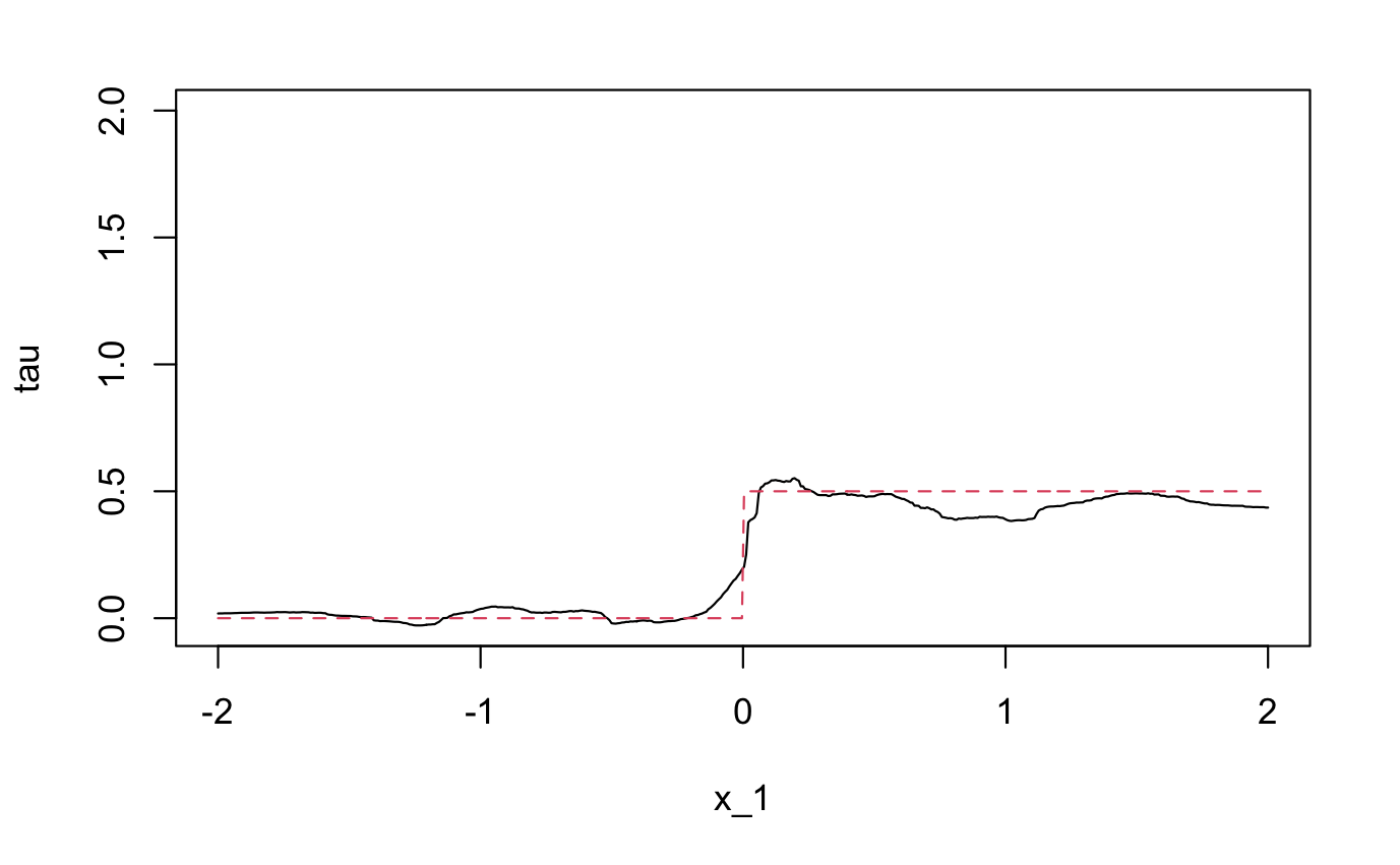 設定1の推定結果
設定2 (アウトカムが2値変数, 介入が連続変数)
介入$W$を連続変数の確率分布(対数正規分布)に置き換えてみる。
\[\begin{align*} & X_1\sim\mathcal{N}(0,1)\\ & X_2\sim\mathrm{Uniform}(0,1)\\ &W\sim \min(\mathrm{LogNormal}(X_1, 1), 1) \\ &Y\sim\mathrm{Bernoulli}(0.5\times W\times\mathbb{I}(X_1 \geq 0)+0.2X_2) \end{align*}\]$W$の分布が異なるだけなので、$\tau(x)$は設定1と同じになる。
シミュレーション
# Generate data.
n <- 2000
p <- 2
n.test <- 500
X <- matrix(0, n, p)
X[, 1] <- rnorm(n)
X[, 2] <- runif(n, min=0, max=1)
X.test <- matrix(0, n.test, p)
X.test[, 1] <- seq(-2, 2, length.out = n.test)
X.test[, 2] <- seq(0, 1, length.out = n.test)

# Train a causal forest.
W <- vapply(rlnorm(n, X[, 1], 1), 1, FUN=function(x) min(x, 1))
Y <- rbinom(n, 1, 0.5 * W * (X[, 1] >= 0) + 0.2 * X[, 2])

tau.forest <- causal_forest(X, Y, W)

# Estimate treatment effects for the test sample.

tau.hat <- predict(tau.forest, X.test)
plot(X.test[, 1], tau.hat$predictions, ylim = range(tau.hat$predictions, 0, 2), xlab = "x_1", ylab = "tau", type = "l")
lines(X.test[, 1], 0.5 * (X.test[, 1] >= 0), col = 2, lty = 2)
予測結果のプロットが以下である。設定1よりは正解からずれてしまったが、ある程度正しく推定できている。
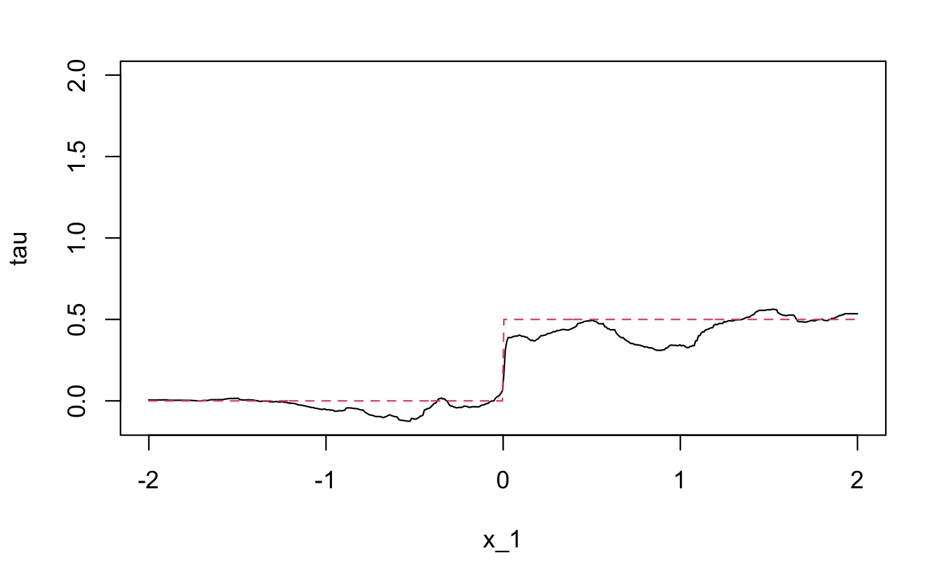 設定2の推定結果
介入が連続変数のときに何を計算しているか
介入が連続変数のとき、tau(x)は何を計算しているのだろうか。Rパッケージのドキュメントのcausal_forestの項をみると、
When W is continuous, we effectively estimate an average partial effect Cov[Y, W | X = x] / Var[W | X = x], and interpret it as a treatment effect given unconfoundedness.
と書いてあるので、average partial effect を推定しているらしい。
同じ質問がgrfのissueに合った。回答としては、Estimating Treatment Effects with Random Forests の式8の $\hat{e}^{(i)}(x)(1-\hat{e}^{(i)}(x))$を$W_i$の条件付き分散$\mathop{\mathsf{Var}}[W_i|X_i]$で置き換えたものを計算しているらしい。
ちなみに式8は以下である。
\[\begin{array}{l} \hat{\tau}_{j}=\frac{1}{n_{j}} \sum_{\left\{i: A_{i}=j\right\}} \widehat{\Gamma}_{i}, \quad \hat{\tau}=\frac{1}{J} \sum_{j=1}^{J} \hat{\tau}_{j}, \quad \hat{\sigma}^{2}=\frac{1}{J(J-1)} \sum_{j=1}^{J}\left(\hat{\tau}_{j}-\hat{\tau}\right)^{2} \\ \widehat{\Gamma}_{i}=\hat{\tau}^{(-i)}\left(X_{i}\right)+\frac{W_{i}-\hat{e}^{(-i)}\left(X_{i}\right)}{\hat{e}^{(-i)}\left(X_{i}\right)\left(1-\hat{e}^{(-i)}\left(X_{i}\right)\right)}\left(Y_{i}-\hat{m}^{(-i)}\left(X_{i}\right)-\left(W_{i}-\hat{e}^{(-i)}\left(X_{i}\right)\right) \hat{\tau}^{(-i)}\left(X_{i}\right)\right) \end{array}\]$W_i$から条件付き平均を引いて条件付き分散で割ることになるので、介入が連続変数のときはtau(x)は$W_i$を標準化したときの介入効果の係数を計算していると考えれば良さそうである。